Excel VBA : Find data using Control+F and not looping

Hi All,

I was sitting and reading few posts and saw that lots of people tries to loop and find the data in different ranges. But it really becomes very very slow if the data you are looping at is huge. Also, what if probability of the occurrences of the desired string/value is very low.

Lets take an example, if I am using approx 1 Million cells in a worksheet, and I am trying to find if a particular text "xysqhqhsyqhsn" is available in how many cells. Obviously, the probability is quite low, and even equal to nil that I will find this string at all in the whole worksheet. But to find, I will need to search first to ensure that the value doesn't exist in the worksheet or not. Now, which option which one would like to have, either to loop to all the 1 million cells or just to jump on the cells which contains the value?

Obviously, in out case, we would like for the second option. I always do that. I always go for the second option to search the string in a worksheet, rather than looping through all the cells, a slow movement.

I have shown an example here. In this example, first I take an input from the user, and tries to give a counter which signifies that the input string exists in how many cells. I have used a function "GetValidRanges" which would return a collection of cells, as shown below

Sub FindInstances()
    Dim inputStr As String ' the variable to accept the input from user
    Dim rngToFind As Range ' the range where we have to find
    Dim activeSht As Worksheet
    Dim cell As Range
    Dim firstAddress As String
    Dim txtCounter As String
    Dim ranges As Collection
    
    'take the input of the string which we want to search.
    
    inputStr = InputBox("Please enter the string which you want to search.")
    Set activeSht = ActiveSheet
    Set rngToFind = activeSht.Range("A1:A300")
    If (inputStr = "") Then
        MsgBox "Invalid Input"
    Else
        'there is a string to search
        Set ranges = GetValidRanges(inputStr, rngToFind)
        
        MsgBox "Total number of occurrences are " & ranges.Count
        
    End If
    
    
    
    
End Sub


'''this function loops through the cells in the range passed, and returns a collection of those cells (eventually range objects) which contains the passed values.

Public Function GetValidRanges(inputStr As String, rngToSearch As Range) As Collection
    Dim cell As Range
    Dim firstAddress As String
    Dim ranges As Collection
    
    Set ranges = New Collection
    
    With rngToSearch
        Set cell = .Find(inputStr, LookIn:=xlValues)
        
        If Not cell Is Nothing Then
            firstAddress = cell.Address
            
            Do
                ranges.Add cell
                Set cell = .FindNext(cell)
            Loop While Not cell Is Nothing And cell.Address <> firstAddress
        End If
    End With
    
    Set GetValidRanges = ranges
    
End Function

User can easily use this collection in many ways. We can get the count of the total cells returned, or loop through all the items in the collection to get the actual address.

Hope this helps :)

Thanks,
Vikas

Dynamic Named Ranges

Hi All,

I see a lot of time people ask that they cannot find the last row of the data. One of the most complicated scenario would be, to assign the dynamic source range to a chart. Suppose I have a chart and the number of rows in my chart would keep on changing time to time, so how would I manage this? One option is to use VBA code and assign a new source data whenever it is refreshed. But do we really need code behind to resolve this problem? I would say no :)

Before going further, I would like to tell you about Offset function, which i will be using to explain the Dynamic named Ranges.

Syntax of Offset function is :

OFFSET(reference,rows,cols,height,width)

Offset, in itself is a powerful function to design a dynamic range.

Parameter 1, Reference : This would be the starting point of your range. Offset function requires you to provide it a starting point, on which you will finally decide what range to be consider.

Parameter 2, Rows : This number is used to shift the starting point. Suppose if the Starting Point is A1, and the number of Rows (second parameter) is 2, then the starting point will be shifted by 2 rows and will point to A3.

Parameter 3, Cols : This number is used to shift the starting point by columns. Suppose if the Starting Point is A1, and the number of columns (third parameter) is 5, then the starting point will be shifted by 5 Columns and will point to F1.

Parameter 4, Height : This would represent the number of cells in a column, aka, the height of range. This can be assumed as the height dimension of a matrix.

Parameter 5, Width : This would represent the width of the range.

Examples :

Offset($A$1,1,1,5,5) : The range is $B$2:$F$6.

Explanation : Starting point is $A$1. Second Parameter, shift row by 1 so It will point to $A$2. As per third Parameter, shift col by 1 so it will point for $B$2. Forth parameter says that the Height of the required range should be 5 cells. So it will be : $B$2:$B$6. The fifth and last parameter says that the width of the range should be 5 columns. So the final range would turn out to be $B$2:$F$6.

Dynamic ranges can be very handy and useful in creating charts when the source range has to be dynamic and is of changing nature. For example, suppose if we have the following chart :



You can see that we have a very simple chart, with the source data as $A$3:$B$11. However, the data can be of a changing nature. For example, see the following screenshot...the data is increased by 5 rows and the new source should be $A$3:$B$16.



Rather than assigning the source data to chart again and again, we can create a Dynamic Named Range which can be flexible if the rows of our data are increased. Dynamic Named Ranges are nothing but a Name Range, with Offset Formula in its target range.

The chart earlier had the series as $A$3:$B$11, if you see and edit the source data of chart, you will see two ranges. One is the Range for Series :- $B$4:$B$11 and X Series which is dates :- $A$4:$A$11.

To create this, I would first create a X Range, which will point to the Date Column of our chart. It will certainly involve the Offset function. To get the dynamic range for Dates, I will start my Offset from $A$4, which is the start point. Setting up next two parameters as 0, 0 so that the starting point should not be changed. Since we have to calculate the rows on run time, so I will use CountA formula so that I can get the exact height of the data. CountA function returns the number of non blank cells in the specified range. Suppose I try CountA($A$4:$A$410) function on the data (as shown in the second image), it would return 13. Because in the entire range (A4:A410) there are only 13 non blank cells. Rest are Blank. Width would be one to ensure that we are talking about a single column(or we can say series or x series values). See the following screenshot :



Similarly, I would create a SharePriceRange



After creating the dynamic named ranges, I will need to assign the name ranges to our chart. In our current chart, we have one series, and one x Series. That is why I have only used two dynamic named ranges. If we will have more series, then we will need to add as many named ranges equal to the number of series present in the chart.

For assigning a named range, I will need to edit the source data. Following is the screenshot of two buttons which we may need to click in order to edit the appropriate series.



The sheet which I am operating is Sheet2, so I will need to ensure that I have included the worksheet name along with the name range. See the two screenshots :








I have created a sample spreadsheet to demonstrate it properly. To download the spreadsheet, please Click here.

Thanks,
Vikas Bhandari

Move the Excel VBA Code from One Workbook to Another.

Hi All,

Recently, I wanted to move VBA Code from one workbook to another. I didn't have any idea. So my teammate did me a favor and got me the following code. So I thought that it is good to share it with the outside world. Moreover, it also moves the code with the Forms as well.

The function expects two parameters,

sourceBook: the workbook where we have to copy the code from
destBook : the workbook where the code has to be copied to

Sub MoveVBACode(sourceBook As Workbook, destBook As Workbook)

    Dim sourceVbComp As VBIDE.VBComponents
    Dim destVbComp As VBIDE.VBComponents


    Dim vbComp As VBComponent


    'To check the code is protected or not
    If sourceBook.VBProject.Protection = vbext_pp_locked Then
        MsgBox "Can't copy code because Source project code is password protected", vbInformation
        Exit Sub
    End If

    Set sourceVbComp = sourceBook.VBProject.VBComponents
    Set destVbComp = destBook.VBProject.VBComponents

    'To copy the modules from source to destination
    For Each vbComp In sourceVbComp
        If vbComp.Type = vbext_ct_Document Then
            CopyModule vbComp, destVbComp, ""
        ElseIf vbComp.Type = vbext_ct_StdModule Then
            CopyModule vbComp, destVbComp, ".bas"
        ElseIf vbComp.Type = vbext_ct_MSForm Then
            CopyModule vbComp, destVbComp, ".frm"
        ElseIf vbComp.Type = vbext_ct_ClassModule Then
            CopyModule vbComp, destVbComp, ".cls"
        End If
    Next

End Sub

Function CopyModule(sourceVbComp As VBIDE.VBComponent, _
                    destVbComp As VBIDE.VBComponents, _
                    extn As String)
    
Dim fName As String
Dim vbComp As VBIDE.VBComponent
Dim destCodeMod As VBIDE.CodeModule
Dim codeText As String
Dim destCodeModule As Variant
Dim TempVBComp As Variant

Const filePath As String = "C:\"
Const xportPath As String = "C:\Temp\"
    
    fName = xportPath & sourceVbComp.Name & extn
    
    sourceVbComp.Export fName
    
    If sourceVbComp.Type = vbext_ct_Document Then
    'To copy the code form ThisWorkbook and sheets
        
        'To get the code module in the destination file
        For Each vbComp In destVbComp
            If vbComp.Type = vbext_ct_Document And vbComp.Name = sourceVbComp.Name Then
                Set destCodeModule = vbComp.CodeModule
                Exit For
            End If
        Next
        
        'To update the code from source to destination
        If Not destCodeModule = "" Then
            Set TempVBComp = destVbComp.Import(fName)
            With destCodeModule
                If TempVBComp.CodeModule.CountOfLines > 0 Then
                     codeText = TempVBComp.CodeModule.Lines(1, TempVBComp.CodeModule.CountOfLines)
                    .InsertLines 1, codeText
                End If
            End With
              destVbComp.Remove TempVBComp
        End If
        
    Else ' For modules ,forms and classes
        destVbComp.Import fName
    End If
        
    'To kill the exported file
    Kill fName

End Function

Thanks,
Vikas

Move all worksheets from a workbook to another

Hi,

Ever moved all the worksheets from a workbook to another. I did it previously, so thought to share the code with you all.

Public Sub CopyWorksheets(sourceBook As Workbook, destBook As Workbook)
   
    Dim shtCounter As Integer
    Dim wkSheet As Worksheet
    
    'remove all the sheets from Destination workbook except one.
    'the last worksheet will be deleted once we have copied the worksheets
    
    For shtCounter = destBook.Worksheets.Count To 2 Step -1
        Set wkSheet = destBook.Worksheets(shtCounter)
        Application.DisplayAlerts = False
        wkSheet.Delete
        Application.DisplayAlerts = True
    Next shtCounter
    
    'rename the sheet1 so that we can assure there is no duplicity
    
    Set wkSheet = Worksheets(1)
    
    wkSheet.Name = "123111xSheet111789" 'giving some arbit name so that we can
                                        ' assure that the sheets we are trying
                                        'copy doesn't have the same name as the worksheet's name.
    
    'copy sheets to destWKB
    
    sourceBook.Worksheets.Copy after:=destBook.Worksheets(1)
    
    
    
    Application.DisplayAlerts = False
    wkSheet.Delete
    Application.DisplayAlerts = True
End Sub

HTH,
Vikas Bhandari

Excel - Break External Links

Hi All,

Please find below the code for Breaking the external links from a Workbook.

Public Sub BreakLinks()
    Dim aLinks As Variant
    Dim i As Integer
    Dim sht As Worksheet
    
    aLinks = ActiveWorkbook.LinkSources(xlExcelLinks)
    If Not IsEmpty(aLinks) Then
        For i = 1 To UBound(aLinks)
            ActiveWorkbook.BreakLink Name:=aLinks(i), Type:=xlExcelLinks
        Next i
    End If
End Sub

Hope this helps.

Thanks,
Vikas

Allow User to Enter Data in a Protected Sheet

Hi All,

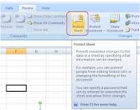
We know that we can protect a worksheet so that user should not able to touch any of values in cell. You can protect the sheet by going to Review Tab --> Protect Sheet option. The option is shown in the following screenshot:



This is easy. But what if we want to allow user to enter data in some of the cells. Or if we want to open few of the cells to the user where he/she can enter his/her inputs.

Protection on a worksheet works only for those cells which are Locked. By default, every cell in a worksheet is locked so when a user protects a worksheet, all of the cells are locked by default. Vice versa, if a cell is not locked then user can edit the data even if the worksheet is protected. So to allow few of the cells to be unlocked(so that these can remain unprotected), we first need to remove the locked option from the cells. Following are the steps given to achieve this :

--> Select the cell which you want to unlock
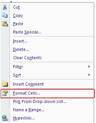
--> Right click on that cell and click on Format Cells. It is displayed in the following screenshot :



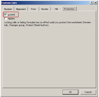
--> Go to the protection Tab, and uncheck the "Locked" option. See the following screenshot:



If you keep this option unchecked for a cell/range, the cell/range cannot be protected. So if you want to keep few of cells open for user in a protected sheet, you can use the above mentioned procedure.

Hope this helps :)

Thanks,
Vikas

Find Last Cell, Column And Row in Excel Worksheet

Hi All,

Please find below a small code snippet, which you can use to find the last Used Cell, Row or Column.

Public Function LastUsedCell() As Range
    Dim rng As Range
    Dim activeSht As Worksheet
    On Error GoTo ErrHandler
    
    Set activeSht = activeSheet

    Set rng = activeSht.Range("A1").SpecialCells(xlCellTypeLastCell)
    
    'return value
    Set LastUsedCell = rng
    Exit Function
ErrHandler:
    Set LastUsedCell = Nothing
End Function

Public Function LastUsedRow() As Long
    Dim rng As Range
    Dim activeSht As Worksheet
    On Error GoTo ErrHandler
    
    Set activeSht = activeSheet

    Set rng = activeSht.Range("A1").SpecialCells(xlCellTypeLastCell)
    
    'return value
    LastUsedRow = rng.Row
    Exit Function
ErrHandler:
    LastUsedRow = 0

End Function


Public Function LastUsedColumn() As Integer
    Dim rng As Range
    Dim activeSht As Worksheet
    On Error GoTo ErrHandler
    
    Set activeSht = activeSheet

    Set rng = activeSht.Range("A1").SpecialCells(xlCellTypeLastCell)
    
    'return value
    LastUsedColumn = rng.Column
    Exit Function
ErrHandler:
    LastUsedColumn = 0

End Function

Hope this helps :)

Thanks,
Vikas

Excel VBA : Loop through all the files and subfolders in a Folder

Hi All,

I write this function many many times in my projects. When we have to create a temporary folder which are specific to our application, then I normally have to loop through all the files in a folder and put some validations so that my code should not replace any previous temp or log files. So I thought to share a small snippet of Excel VBA code where I am trying to search all the files in a Folder ( and its subfolders too) and printing in an Excel Worksheet.

Private fileCounter As Integer
Private activeSht As Worksheet
'Display all the files in a folder. Searches all the sub folders.

'Prints Folder Names in Column A and and the file Names in Column B

Sub SearchFiles()
    Dim pth As String
    Dim fso As FileSystemObject
    Dim baseFolder As Folder
                    
    pth = "C:\Projects\" 'the base path which has to be searched for Files
    Set fso = New FileSystemObject
                    
    ''check if the folder actually exists or not
                    
    If (Not (fso.FolderExists(pth))) Then
        'the folder path is invalid. Exiting.
        MsgBox "Invalid Path"
        Exit Sub
    End If
    
    Set baseFolder = fso.GetFolder(pth)
    
    fileCounter = 1
    Set activeSht = ActiveSheet
    
    activeSht.Range("A1").Value = "Folder Name"
    activeSht.Range("B1").Value = "File Name"
    
    On Error GoTo ErrHandler
    Application.ScreenUpdating = False
    Application.Calculation = xlCalculationManual
    PrintFileNames baseFolder
    
ErrHandler:
    Application.ScreenUpdating = True
    Application.Calculation = xlCalculationAutomatic
End Sub
    
    
Sub PrintFileNames(baseFolder As Folder)
    Dim folder_ As Folder
    Dim file_ As File
    
    For Each folder_ In baseFolder.SubFolders
        'call recursive function.
        PrintFileNames folder_
    Next folder_
    
    For Each file_ In baseFolder.Files
        'print files here
        activeSht.Range("A1").Offset(fileCounter, 0).Value = baseFolder.Path
        activeSht.Range("B1").Offset(fileCounter, 0).Value = file_.Name
        fileCounter = fileCounter + 1
    Next file_
End Sub
    

The above code loops through all the subfolders and the files in a given folder and prints the folder names in Column A and the file Names in Column B.

HTH,
Vikas

Write Custom Functions in Excel.

Hi,

We all know that we can write Formulas in Excel. for example, =Sum(A1:A10) to sum the values present in range from A1 to A10. The summation is easy. Right??? But what if we want to tweak our requirements.

Let's assume we have a requirement, that we need to sum only those values which are divisible by 2. I have assumed a very basic example, although we can write an Excel Built in for this requirement, but I want to show to achieve this through Custom Function.

For example, I want to sum range A1 to A10. I will write a custom Function in Excel VBA. Open VBA editor, add Module 1 and add a function like following :

Public Function SumEvenValues(rng As Range) As Double
    Dim sum As Double
    Dim cell_ As Range
    
    sum = 0
    
    For Each cell_ In rng.Cells
        If (IsNumeric(cell_.Value)) Then
            'the value is numeric. Check the mod
            If (cell_.Value Mod 2 = 0) Then
                sum = sum + cell_.Value
            End If
        End If
    Next cell_
    
    SumEvenValues = sum
    
End Function

In your excel workbook, in Cell b1, type this : =SumEvenValues(A1:A10)

You will see that all the values which are divisible by 2 are summed up and the result is displayed in Cell B1. I have taken a very basic example to show it's use, which can be easily achived in Excel, but we may encounter to include those requirements which we may not be able to achieve within Excel only. So in such a case, VBA is used to handle all those requirements which Excel cannot handle.

HTH,
Vikas

Linking Two Pivot Tables

Hi all,

Recently, I was making a dashboard and I had to create two Pivot Tables. My conditional formatting was set in such a manner, that I needed to have both the pivot tables updated @ same time, and the items too, to be shown or hid @ the same time in both the pivot table.

To achieve this, I first noted down the fields which I had to filter. I had three fields to filter and these items were Name, Date, and Month. So I had to make the following code :


Private Sub Worksheet_PivotTableUpdate(ByVal Target As PivotTable)
'ExpectedHours

If (Target.Name = "MainPivot") Then
      Macro1
End If

End Sub

Sub Macro1()
'

'
'On Error Resume Next
'
      Dim pivotSource As PivotTable
      Dim pivotTarget As PivotTable
      Dim sourceItem As PivotItem
      Dim sourceField As PivotField
      Dim targetItem As PivotItem
      Dim targetField As PivotField
      
      Set pivotSource = Sheet7.PivotTables("MainPivot")
      Set pivotTarget = Sheet7.PivotTables("ExpectedHours")
      
      
    Set targetField = pivotTarget.PivotFields("department")
   
    targetField.ClearAllFilters
    targetField.CurrentPage = Sheet7.Range("Department").Value
   
   
    Set sourceField = pivotSource.PivotFields("Name")
    Set targetField = pivotTarget.PivotFields("Name")
   
    For Each sourceItem In sourceField.PivotItems
            
            Set targetItem = GetPivotItemByName(targetField, sourceItem.Name)
            
            If (Not (targetItem Is Nothing)) Then
            
                  If (targetItem.Visible <> sourceItem.Visible) Then
                        targetItem.Visible = sourceItem.Visible
                  End If
            End If
    Next sourceItem
      
      
    Set sourceField = pivotSource.PivotFields("Date")
    Set targetField = pivotTarget.PivotFields("Date")
   
    For Each sourceItem In sourceField.PivotItems
            
            Set targetItem = GetPivotItemByName(targetField, sourceItem.Name)
            
            If (Not (targetItem Is Nothing)) Then
            
                  If (targetItem.Visible <> sourceItem.Visible) Then
                        targetItem.Visible = sourceItem.Visible
                  End If
            End If
    Next sourceItem
      
            
    Set sourceField = pivotSource.PivotFields("Month")
    Set targetField = pivotTarget.PivotFields("Month")
   
    For Each sourceItem In sourceField.PivotItems
            
            Set targetItem = GetPivotItemByName(targetField, sourceItem.Name)
            
            If (Not (targetItem Is Nothing)) Then
                  If (targetItem.Visible <> sourceItem.Visible) Then
                        targetItem.Visible = sourceItem.Visible
                  End If
                  
                  If (targetItem.ShowDetail <> sourceItem.ShowDetail) Then
                        targetItem.ShowDetail = sourceItem.ShowDetail
                  End If
            End If
    Next sourceItem
End Sub


Public Function GetPivotItemByName(field As PivotField, item As String) As PivotItem
      On Error Resume Next
      Dim pvItem As PivotItem
      
      Set pvItem = Nothing
      
      Set pvItem = field.PivotItems(item)
      
      Set GetPivotItemByName = pvItem
End Function

Hope this helps :)

Thanks,
Vikas

Back to XL VBA : A Way to create Utility functions to increase reusability

Hi there!

I normally create a Util Module every time I work on an Office Automation Project. I thought, people may be benefitted with it. Moreover, I will not have to create it again. I will copy it from here only ;)

Public Function SheetExists(wkb As Workbook, shtName As String) As Boolean
    Dim sht As Worksheet
    
    Set sht = Nothing
    On Error GoTo errHandler
    Set sht = wkb.Worksheets(shtName)
    SheetExists = True
    Exit Function

errHandler:
    SheetExists = False
End Function

Public Function GetSheet(wkb As Workbook, shtName As String) As Worksheet
    Dim sht As Worksheet
    
    Set sht = Nothing
    If (SheetExists(wkb, shtName)) Then
        Set sht = wkb.Worksheets(shtName)
    End If
    
    Set GetSheet = sht
End Function


Public Function RangeExists(wkSht As Worksheet, rngName As String) As Boolean
    Dim rng As Range
    
    Set rng = Nothing
    On Error GoTo errHandler
    Set rng = wkSht.Range(rngName)
    RangeExists = True
    Exit Function

errHandler:
    RangeExists = False
End Function

Public Function GetRange(wkSht As Worksheet, rngName As String) As Range
    Dim rng As Range
    
    Set rng = Nothing

    If (RangeExists(wkSht, rngName)) Then
        Set rng = wkSht.Range(rngName)
    End If
    
    Set GetRange = rng
End Function


Public Function GetRows(wkSht As Worksheet, Optional columnName As String = "A") As Long
    Dim rowCounter As Long
    Dim runLoop As Boolean
    Dim startRange As Range
    
    rowCounter = 0
    runLoop = True
    
    Set startRange = wkSht.Range(columnName & "1")
    
    While runLoop
        If (Len(startRange.Offset(rowCounter, 0).Value) > 0) Then
            rowCounter = rowCounter + 1
        Else
            runLoop = False
        End If
    Wend
    
    GetRows = rowCounter
    
End Function

Public Function GetColumns(wkSht As Worksheet, Optional rowNum As String = "1") As Long
    Dim colCounter As Long
    Dim runLoop As Boolean
    Dim startRange As Range
    
    colCounter = 0
    runLoop = True
    
    Set startRange = wkSht.Range("A" & rowNum)
    
    While runLoop
        If (Len(startRange.Offset(0, colCounter).Value) > 0) Then
            colCounter = colCounter + 1
        Else
            runLoop = False
        End If
    Wend
    
    GetColumns = colCounter
    
End Function

Thanks,
Vikas

Designing a Button in WPF - "Simplest yet cool Button"

Hi All,

I have seen a lot of button templates which offer a cool looking styles by overriding the complete button template. Just to give a small style to a button can be complicated as far as overriding the template is concerned. I tried to build a button something like this :



An option could be, to include a new style for my button and override the template. But do we really need to do that???? I don't think so. The button which you are seeing in the Image is actually not a button, it is actually a border object filled with Alice Blue color, and with the corner radius set to 5. There is a textblock object inside the border so that it can contain some text. I didn't use label for that because textblock is lighter than a label.




Now, this control is not yet completed because it doesn't give any notification whenever it is clicked. So I had to include some animation to this button.




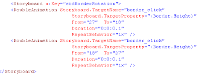
Here, I have opted to use code behind to run my animation. Like shown in the figure below :




After including the above code lines, you can see that the border looks like a button and animates as well once you click the control.

HTH,
Vikas